HyperSpace

Distributed Bayesian Optimization

Bayesian Optimization

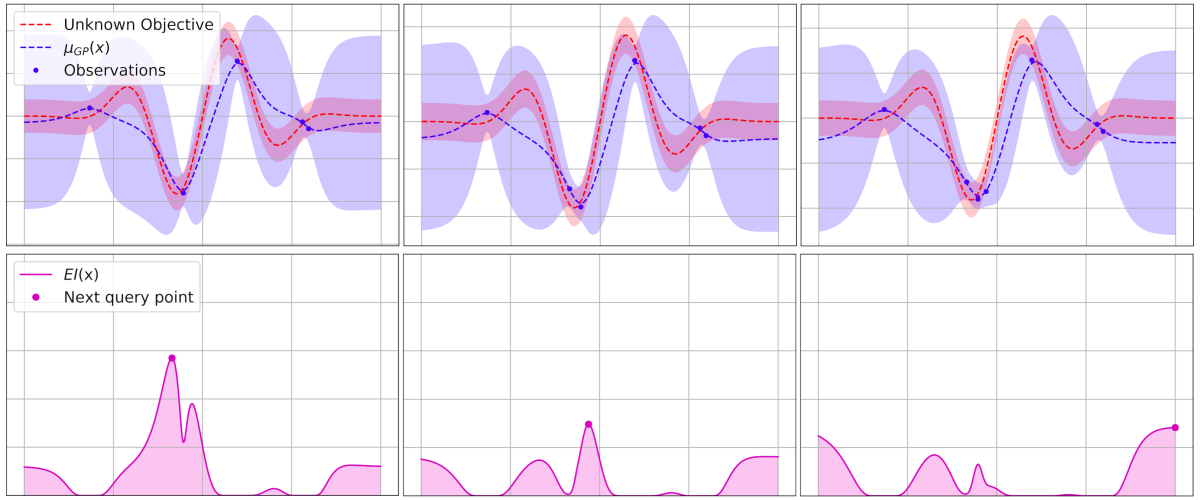
1. Sample a small, predefined number of, typically \(n=10\) points \(x_i\in X\), uniformly randomly, and compute the function values at those locations, \(f(x_1), \ldots, f(x_n)\).

2. We then model \(f\) by fitting a probabilistic model for the function. Here we assume that \(f\) is drawn from a Gaussian process.

3. We then must decide where to sample our next point, \(x_{n+1}\), from \(X\) as we seek the location of the function's minimum. This is controlled by a proxy optimization of an acquisition function* \(u:X\rightarrow \mathbb{R^{+}}\):

x_{n+1} = \arg\max_x \enskip u(x)

x_{n+1} = \arg\max_x \enskip u(x)

Bayesian Optimization

Limitations of Bayesian Optimization

1. Sequential by nature.

2. Exponential scaling.

The number of samples required to bound our uncertainty about the optimization procedure is scales exponentially with the number of search dimensions, as in \(2^{D}\), where \(D\) is number of dimensions [1, 2]. This has been forgotten in the recent excitement of Bayesian optimization.

1. N. Srinivas, A. Krause, S. M. Kakade, and M. W. Seeger. Gaussian process bandits without regret: An experimental design approach. CoRR, abs/0912.3995, 2009.

2. S. Grunewalder, J.-Y. Audibert, M. Opper, and J. Shawe-Taylor. Regret Bounds for Gaussian Process Bandit Problems. In AISTATS 2010 - Thirteenth International Conference on Artificial Intelligence and Statistics, volume 9, pages 273–280, Chia Laguna Resort, Sardinia, Italy, May 2010.

HyperSpace Approach

1. Parallelism that focuses on the search space.

2. Build many surrogate functions in parallel.

3. Prayer.

Partitioning

the

search

space

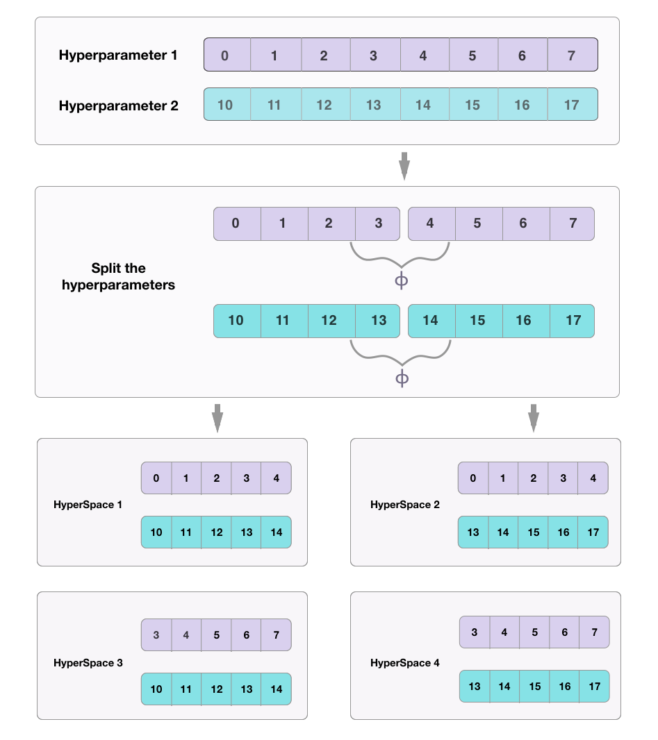
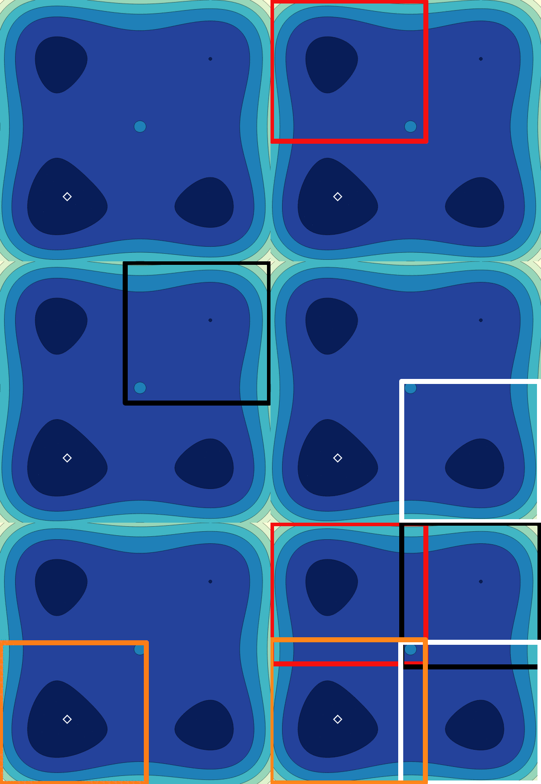
Partitioning the Search Space

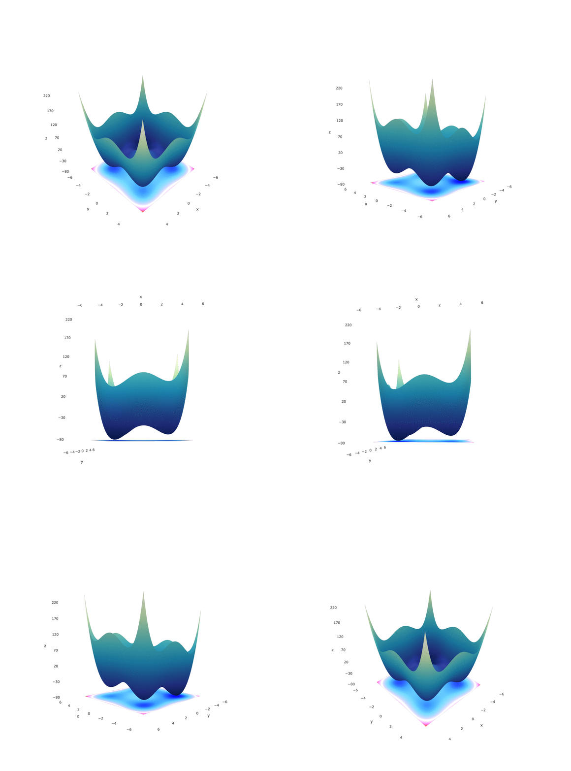
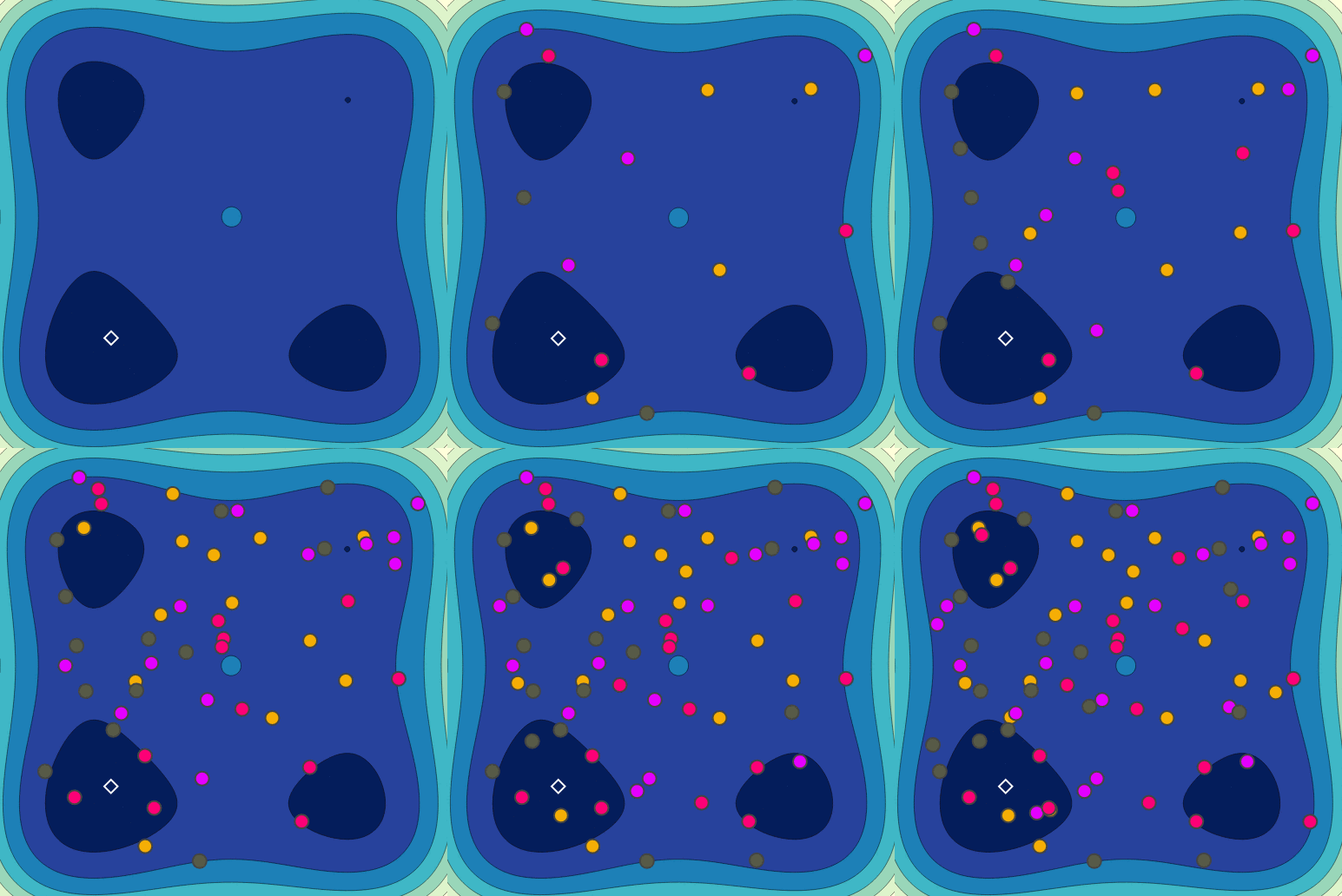
Styblinski-Tang Function

Random Search

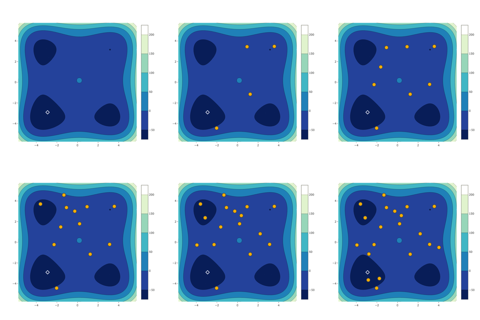
Bayesian Optimization

HyperSpace

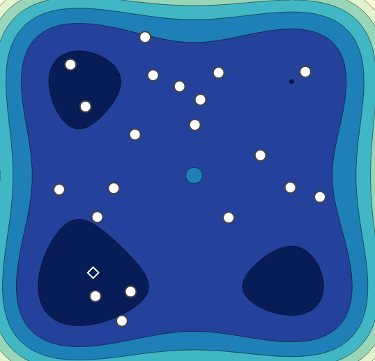
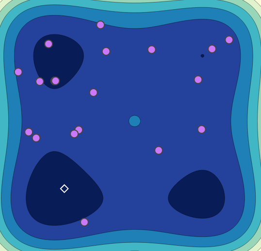
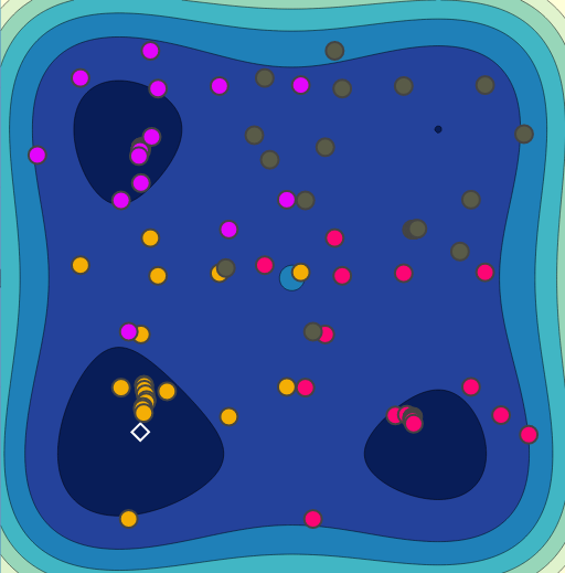
Random Search

Bayesian Optimization

HyperSpace

Sample Comparison

 from hyperspace import hyperdrive


 def objective(params):
     """
     Objective function to be minimized.
     """
     param0, param1, param2 = params
     model = Model(param0, param1, param3)

     train_loss = train(model)
     val_loss = validate(model)

     return val_loss


 def main():
     hparams = [(2, 10),             # param0
                (10.0**-2, 10.0**0), # param1
                (1, 10)]             # param2

     hyperdrive(objective=objective,
                hyperparameters=hparams,
                results_path='/path/to/save/results',
                model="GP",
                n_iterations=15,
                verbose=True,
                random_state=0,
                sampler="lhs",
                n_samples=5,
                checkpoints=True)


 if __name__ == '__main__':
     main()

HyperSpace is Open Source

https://github.com/yngtodd/hyperspace

References

1. N. Srinivas, A. Krause, S. M. Kakade, and M. W. Seeger. Gaussian process bandits without regret: An experimental design approach. CoRR, abs/0912.3995, 2009.

2. S. Grunewalder, J.-Y. Audibert, M. Opper, and J. Shawe-

Taylor. Regret Bounds for Gaussian Process Bandit Problems. In AISTATS 2010 - Thirteenth International Conference on Artificial Intelligence and Statistics, volume 9, pages 273–280, Chia Laguna Resort, Sardinia, Italy, May 2010.

3. Li, K. Jamieson, G. DeSalvo, A. Rostamizadeh, and A. Talwalkar. Hyperband: A novel bandit-based approach to hyperparameter optimization. In International Conference on Learning Representations (ICLR2017). CBLS, April 2017

Supplemental Material

x_{n+1} = \arg\max_x \enskip u(x)

x_{n+1} = \arg\max_x \enskip u(x)

Bayesian Optimization in Detail

1. Sample a small, predefined number of, typically \(n=10\) points \(x_i\in X\), uniformly randomly, and compute the function values at those locations, \(f(x_1), \ldots, f(x_n)\).

2. We then model \(f\) by fitting a probabilistic model for the function. Here we assume that \(f\) is drawn from a Gaussian process.

The acquisition function balances two competing aims: the need to explore the domain of our objective function and the desire to exploit points on the domain which may be the global minimum of the function. By default, HyperSpace uses the Expected Improvement function, but there are several options available.

Acquisition Functions

Expected Improvement:

u_{EI}(x) = E \left[\max \left(0, \enskip f(x^{*})-f(x) \right) \right]

u_{EI}(x) = E \left[\max \left(0, \enskip f(x^{*})-f(x) \right) \right]

where \(f(x^{*})\) is the minimal observed value of \(f\) thus far and \(E[\cdot]\) denotes expectation over the random variable \(f(x)\). We therefore receive a reward equal to the "improvement" \(f(x^{*}) - f(x)\) when \(f(x)\) is less than \(f(x^{*})\), and no reward otherwise. Given the GP's predictive mean and variance functions, the right hand side of the above equation can be re-expressed as

u_{EI}(x) = (f(x^*)-\mu(x)) \Phi \left( Z\right) + \phi(Z)

u_{EI}(x) = (f(x^*)-\mu(x)) \Phi \left( Z\right) + \phi(Z)

where \(\Phi\) is the standard normal cumulative distribution function, \(\phi\) is its derivative, and \(Z = \frac{f(x^{*}) - \mu(x)}{\sigma(x)}\).

Parallel Random Search

Parallel Random Search

HyperSpace

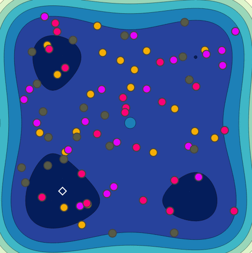
Sample Comparison